Activity 12 – Color Image Processing

The aim of this activity is to compare the White Patch algorithm and the Gray World algorithm in balancing and improperly captured image under an unmatched white balancing set-up. This means that for an imbalanced image, white is seen differently from white per se and so are other colors and opposite happens when the image is balanced.Now, from an image of red, green and blue put on a white paper under a constant illumination but captured under different white balance modes of the camera, I chose what the ones which are improperly balanced and applied the two balancing algorithms to it. The images shown below are the captured images using the same camera but under various white balance modes. The last three pictures are the imbalanced ones.

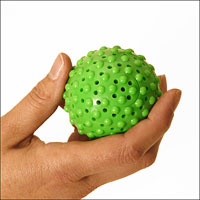
So at this point, the last three images will be our concern. Using the White Patch algorithm wherein i chose a small part of the background which is supposedly a white bond paper then arbitrarily choose a point on it that will serve as the divisor for the pixel values of R,G,B of the image. After applying a scaling factor differently for each layer of R,G and B, I clipped the maximum value to be 1 by saturating those which exceeds one. The images below is the result of the first algorithm applied to the last three images above in the same order.

We can observe the difference in quality of the balanced image, nevertheless, it significantly improved as compared to its original form above.

Now, we apply the Gray World algorithm to the same images and see what happens. This algorithm, by the way, just replaces the divisor of the R,G,B layers of the imbalanced image with the average of each layer. Everything else follows the same procedure.

There is not much difference in the quality of the balanced images for three different WB camera modes. However, we can see that the new image is like exposed to a higher intensity light source. There is not much difference in rendered colors especially the white background unlike the first algorithm where there is much distinction between the white backgrounds.

Going to another imbalanced image with largely the same hue (in this case green) and the applying the two algorithms, we get the results below.

Imbalanced image

Balanced using White Patch algorithm

Balanced using Gray World algorithm

The most properly balanced image in this case is the one using White Patch algorithm. We observe here the same effect that the second algorithm produced with first set of images. It intensifies the white value in the image and it appears now that the object image was capture under a very high intensity white light source. Also from the procedure done in the algorithm, one can infer that White Patch algorithm depends solely on a single white value in the image while the Gray World algorithm depends entirely on the colors of the captured image since it relies it divisor value from the mean of all values. The best algorithm, well for this case in the first one.

This activity compared to other ones is relatively easy but its application is noble and dynamic. The concept was well understood and the procedures executed smoothly. It is just to give myself a grade of 9 for this one.

Activity 3 – Image Types and Formats

An example of a grayscale image

Following the procedures in this activity, I opened my scanned image from activity1 and found out that it is a grayscale image. It is grayscale since the image is not in three layer of R,G and B but pixels have numbers ranging from 45 to 256. The image is shown above. Its size is 1221×967 or 1180707 bytes or 1.2MB.

Now, getting each of the basic and advanced image types:

An example of binary image

grayscale image

truecolor image

indexed image

Choosing a truecolor image, which is the image of an elephant, and transforming it to binary and grayscale. We produce the same dimensions but only the 3 layers from RGB are removed. The dimension are both 432×550. Image is shown below.

(from left to right) binary & grayscale of a truecolor image

Now, from the graph in activity1 we extract the grayscale valuesof the image and its frequancy by getting its histogram. Once this information is known, we can binarize the image to make the points in the graph more distinct. The histogram and the choice of grayscale value to establish threshold is shown below with the resulting binary image.We note here that we first scaled the grayscale image of values from 0-255 t0 0-1 by dividing the maximum value to each pixel of the image. Then we get its histogram. The lighter colored pixels occupy most of the area in the graph. So we begin to binarize at around 0.3 value. The resulting image is shown. Although, there can be no clearer separation of the data points from the grid lines since they have common pixel values.

There is little effort done for this activity. And honestly, this activity was the most unliked one since it took me almost a semester to do it. I wasn’t able to finish the activity. I deserve a grade of 6 for this output.

Activity 13 – Color Image Segmentation

The aim of this activity is to separate a region of interest(ROI) among all the objects in a given image. For an easier implementation of this, it is suggested that the ROI possess a single color. The image I used is shown below with ROI cropped.

The first thing to do here is to crop out the monochromatic region of interest which is the green spiky ball. Then I get the normalized chromaticity coordinates by dividing each R,G and B values in the matrix by their corresponding sum of both the entire image and the ROI. Then before obtaining the probability that the r and g values of every pixel belong to the ROI(p(r) and p(g) respectively, I first obtained the mean and standard deviation of the R and G matrix of the entire image since they values are relevant to the probability distribution.

After applying the probability distribution on each R and G matrix, we get the following images.

(From left to right) P(r) and P(g)

The closer to white pixels suggests that there is a very high probability that those areas would belong to ROI, otherwise they are of less importance with respect to the ROI. If we multiply both of these images we get the figure below.We can still observe here that even though the hand is of less importance with respect to the ROI, the white background still contains green values to it so that it is slightly close in color to the spiky ball. To further remove the white as belonging to the ROI, I binarized the image. It is now shown below.

Notice here the entire separation of the spiky ball with the white background.

Now, using another technique of ROI separation, we first make a 2D histogram of the original image by just following the code presented in Mam Jing’s lecture. We also compare the derived histogram with the rg chromaticity diagram. This is shown below.

We take note here that the histogram is rotated 90degress CCW so that their origins will be the same. We can observe that area where non-zero values are found is located in the greenish part of the rg chromaticity diagram like we espected since we get the histogram of a green spiky ball. The histogram by the way is 32x32pixels. Now, like in the backprojection of the previous activity, we are to translate to the image the histogram the histogram shown. This is done by getting the r & g values of the original image. These values just range from 0-1, and since we are to locate it in the histogram, we must first rescale it from 1-32. It is very important to note here that the value of zero for the r and g is prohibited since they will serve as pixel locations in the histogram. What I did was to convert all zeros to one.Now, I took the value of the rescaled r as the x-axis of my histogram and rescaled g as the y-axis. If there are 200×200 values of r’s and g’s, then there will also be 200×200 points from the histogram values which I will place in the same position as my r and g. Upon doing this, i get the image below.

We can stll see here that ROI encompasses even the background since it is white. The problem here is that although there is some degree of distinction between the white background and the ball but since it peaked out into the white parts thresholding will be difficult.But then I still can clearly separate it from the background by translating the values of the background into near zero or zero itself.

I guess the first part ROI separation is easier to code and gives a reliable result. Still, the second approach is good but i had a hard time doing it so that I obtained this bias. Anyway, I thank mam for helping me in figuring out and debugging the code for my histogram backprojection.

It would be fair enough to give myself a grade of 9 for this activity since all concepts had been clear to me. Only that small programming details have been ignored by oversimplification of concept.

Activity 14 – Image Compression

In this activity, I will be compressing the image of  water lilies which i got from the sample pictures of  my computer. This is essentially an RGB image, and it was converted to grayscale by adding up the matrix of red, green and blue and dividing it by the maximum of these three values which is 3. The original RGB and the grayscale conversion is presented below.

RGB image

grayscale image

From the grayscale image of size 600×800, it was partitioned into 10×10 matrices which now becomes 60×80, 10×10 matrices. Code is shown.

k=0;
for r = 1:60
for c = 1:80
itemp = I(((10*r-9):(10*r)),((10*c-9):(10*c)));
xtemp = itemp(:);
k = c+(r-1)*80;
x(k,:) = xtemp’;
end;
end;

Then the image x is applied to a pca function in order to get the desired number of lambdas to used for compression. The lambda contribution I chose accumulated to about 95.7% or the first 7 lambdas. Also from this function, we get the ‘basis vectors’ of the image which is also 10×10 in size and from the code, there are a hundred of them. From the information of the number of lambdas to use, I only used the same amount of ‘basis vectors’ to reconstruct the image. PCA code is presented.

[lambda,facpr,comprinc] = pca(x);

y = zeros(100,100);
k=0;
for r=1:10
for c = 1:10
k = c+(r-1)*10;
xtemp = facpr(:,k);
y((10*r-9):(10*r),((10*c-9):(10*c))) = matrix(xtemp,10,10);
end;
end;
//scf(); imshow(y);

Then, from those 7 ‘eigenvectors’, I multipiled the partitioned imaged to each of the eigenvectors and obtained its corresponding sum. This is basically getting the dot product. These numbers or the eigenvalues are stored in a hypermatrix of 7 layers; each layer is obviously 60×80 in size. Code is presented.

hyper_matrix =hypermat([60,80,7]);
for h=1:7
for z=1:60
for a=1:80
new_matrix = I(((10*z-9):(10*z)),((10*a-9):(10*a))).*(y(1:10,((10*h-9):(10*h))));
hyper_matrix(z,a,h) = sum(new_matrix);
end;
end;
end;

From the hypermatrix made, each of the layers having the same location is multipied to the eigenvectors. Then they are summed up and this represents now the 10×10 subimage of the water lilies. The corresponding position in the hypermatrix is the position of the summed vectors in the reconstruction of the image. Dimensionally this is correct since there are 60×80 10×10 ‘s in the original water lily image and so there are also 60×80 in each layer of hypermatrix and the multiplied object(eigen vector) is 10×10 in size. So, bringing the size back to 600×800. Code is shown.

x_comp = [];

for m=1:60
for n=1:80
simple_matrix = zeros(10,10);
for l=1:7
simple_matrix = simple_matrix+hyper_matrix(m,n,l)*(y(1:10,((10*l-9):(10*l))));
x_comp(((10*m -9):(10*m)),((10*n-9):(10*n))) = simple_matrix;
end;
end;
end;

imshow(x_comp);

The resulting compressed image is presented.

Compressed grayscale

We can see that the quality of the picture is reduced and so is the memory size. We can compute the pecent compression by first knowing the number of elements used in the eigenvectors, in this case, it is 7 times a hundred(700) then, also we must know the number of subimages that the images was partitioned, and in this case it amounted to 60×80, 0r 4800 multiplied by the amount of eigenvalues used per subimage which is seven(7). When we add the two up, we get a value of 34300. The original size of the image is basically the number of pixels it has, it amounted to 600×800 or 480000. Therefore the percent compression obtained in this activity is 34300/480000 or we are able to compress the image by up to 7% its original size.

I tried different approaches during my reconstruction part and this approach takes the least amount of code and so in the same way I was able to compress my code. I would probably deserve a grade of 10 for this. However, I must admit that I copied the image presented by Mam Jing in her lecture. This is convenient since the size is divisible to a 10×10 matrix.

In this activity, which was really lengthy but enjoyable in a way, a simple musical piece is selected and by applying image processing to it scilab will be able to know the tune and the tempo of every note on the staff. The song i selected was timely and it is entitled “Jingle Bells”. I only cropped the chorus part of the song. The image is shown.

Part of the Jingle Bells chorus which will be played in scilab

The first thing i did here was to get the binarized version of the image above and thresholding it to 0.75 of grascale value so that each note is still distinguishable. Next, i cropped every type of note in the piece like half note & quarter note. Then, using the correlation function from the previous activity I was able to find where will each kind of note will be found in the staff. Then I binarized each of the correlated image so that a single pixel will appear for every corresponding note. And before adding up all those images in a single image, I first distinguished every type of note from the rest by asigning a numerical value to it. I already proportioned its number with its timing i.e. for half note is 4, for quarter its 2 etc. Now, i summed all of them to produce a single image presenting in the same order of notes the relative tempo of every note in the staff. Code is presented below:

//GETTING THE TEMPO OF THE NOTES
quarter_note = imread(‘D:\academic documents\1st sem AY 10-11\AP 186\Activity_11\quarter_note.jpg’);
quarter_note = im2bw(quarter_note,0.75);
//imshow(quarter_note);

conj_fft_jingle = conj(fft2(jingle_bells));
fft_quarter = fft2(quarter_note);
convlv_in_fft1 = conj_fft_jingle.*fft_quarter;
correlation1 = abs(fftshift(fft2(convlv_in_fft1)));
correlation1 = (correlation1-min(correlation1))/(max(correlation1)-min(correlation1));
//imshow(correlation);
//histplot(100,correlation);
T_new1 = im2bw(correlation1,0.9);
//imshow(T_new1);
imwrite(T_new1,’correlation_with_quarter.jpg’)

half_note = imread(‘D:\academic documents\1st sem AY 10-11\AP 186\Activity_11\half_note.jpg’);
half_note = im2bw(half_note,0.75);

fft_half = fft2(half_note);
convlv_in_fft2 = conj_fft_jingle.*fft_half;
correlation2 = abs(fftshift(fft2(convlv_in_fft2)));
correlation2 = (correlation2-min(correlation2))/(max(correlation2)-min(correlation2));
//imshow(correlation);
//histplot(100,correlation);
T_new2 = im2bw(correlation2,1.0);
//imshow(T_new2);
imwrite(T_new2,’correlation_with_half.jpg’)

eighth_note = imread(‘D:\academic documents\1st sem AY 10-11\AP 186\Activity_11\eighth_note.jpg’);
eighth_note = im2bw(eighth_note,0.75);

fft_eighth = fft2(eighth_note);
convlv_in_fft3 = conj_fft_jingle.*fft_eighth;
correlation3 = abs(fftshift(fft2(convlv_in_fft3)));
correlation3 = (correlation3-min(correlation3))/(max(correlation3)-min(correlation3));
//imshow(correlation);
//histplot(100,correlation);
T_new3 = im2bw(correlation3,1.0);
//imshow(T_new3);
imwrite(T_new3,’correlation_with_eighth.jpg’)

half_eighth_note = imread(‘D:\academic documents\1st sem AY 10-11\AP 186\Activity_11\half+eighth_note.jpg’);
half_eighth_note = im2bw(half_eighth_note,0.75);

fft_half_eighth = fft2(half_eighth_note);
convlv_in_fft4 = conj_fft_jingle.*fft_half_eighth;
correlation4 = abs(fftshift(fft2(convlv_in_fft4)));
correlation4 = (correlation4-min(correlation4))/(max(correlation4)-min(correlation4));
//imshow(correlation);
//histplot(100,correlation);
T_new4 = im2bw(correlation4,1.0);
//imshow(T_new4);
imwrite(T_new4,’correlation_with_quarter&eighth.jpg’)

half_quarter_note = imread(‘D:\academic documents\1st sem AY 10-11\AP 186\Activity_11\half+quarter_note.jpg’);
half_quarter_note = im2bw(half_quarter_note,0.75);

fft_half_quarter = fft2(half_quarter_note);
convlv_in_fft5 = conj_fft_jingle.*fft_half_quarter;
correlation5 = abs(fftshift(fft2(convlv_in_fft5)));
correlation5 = (correlation5-min(correlation5))/(max(correlation5)-min(correlation5));
//imshow(correlation);
//histplot(100,correlation);
T_new5 = im2bw(correlation5,1.0);
//imshow(T_new5);
imwrite(T_new5,’correlation_with_half&quarter.jpg’)

//PUTTING TEMPO TO THE PIECE
jingle_bells_quarter = imread(‘D:\academic documents\1st sem AY 10-11\AP 186\Activity_11\correlation_with_quarter.jpg’);
jingle_bells_quarter = (jingle_bells_quarter – min(jingle_bells_quarter))/(max(jingle_bells_quarter)-min(jingle_bells_quarter));
jingle_bells_quarter = im2bw(jingle_bells_quarter,0.9);
//y = tabul(jingle_bells_quarter);
//imshow(jingle_bells_quarter);
jingle_bells_quarter = 2*jingle_bells_quarter;

jingle_bells_half = imread(‘D:\academic documents\1st sem AY 10-11\AP 186\Activity_11\correlation_with_half.jpg’);
jingle_bells_half = (jingle_bells_half – min(jingle_bells_half))/(max(jingle_bells_half)-min(jingle_bells_half));
jingle_bells_half = im2bw(jingle_bells_half,0.9);
//y = tabul(jingle_bells_half);
jingle_bells_half = 4*jingle_bells_half;

jingle_bells_eighth = imread(‘D:\academic documents\1st sem AY 10-11\AP 186\Activity_11\correlation_with_eighth.jpg’);
jingle_bells_eighth = (jingle_bells_eighth – min(jingle_bells_eighth))/(max(jingle_bells_eighth)-min(jingle_bells_eighth));
jingle_bells_eighth = im2bw(jingle_bells_eighth,0.9);
//y = tabul(jingle_bells_eighth);
//imshow(jingle_bells_eighth);
jingle_bells_eighth = 1*jingle_bells_eighth;

jingle_bells_half_q = imread(‘D:\academic documents\1st sem AY 10-11\AP 186\Activity_11\correlation_with_half&quarter.jpg’);
jingle_bells_half_q = (jingle_bells_half_q – min(jingle_bells_half_q))/(max(jingle_bells_half_q)-min(jingle_bells_half_q));
jingle_bells_half_q = im2bw(jingle_bells_half_q,0.9);
//y = tabul(jingle_bells_half_q);
jingle_bells_half_q = 6*jingle_bells_half_q;

jingle_bells_quarter_e = imread(‘D:\academic documents\1st sem AY 10-11\AP 186\Activity_11\correlation_with_quarter&eighth.jpg’);
jingle_bells_quarter_e = (jingle_bells_quarter_e – min(jingle_bells_quarter_e))/(max(jingle_bells_quarter_e)-min(jingle_bells_quarter_e));
jingle_bells_quarter_e = im2bw(jingle_bells_quarter_e,0.9);
//y = tabul(jingle_bells_quarter_e);
jingle_bells_quarter_e = 3*jingle_bells_quarter_e;

new_jingle_bells = jingle_bells_quarter + jingle_bells_half + jingle_bells_eighth + jingle_bells_half_q + jingle_bells_quarter_e;
//t = tabul(new_jingle_bells);
//imshow(new_jingle_bells);

Now, the next problem was to find the corresponding tune for every note and this can be done by finding the height/column correspondence to every note in the staff. However, our last image was only for tempo information since the peaks of the correlation do not always dwell on the middle part of the oblong head of the note and it depends on the shape of the entire note i.e. including the tail, the flags and dots beside it. So, a different approach is required. What i did was to create different sizes of oblongs in paint and used morphological closing and opening as well as twice erosion process in order to remove hollow oblongs from half note, tails and flags from lower tempo notes as well as the lines of the staff and to reduce the oblong heads into few pixels. I find the correspondence of column value to the conventional positions of tunes of notes on the staff. Code is presented:

//FOR DETERMINING THE TUNE
jingle_bells = imread(‘D:\academic documents\1st sem AY 10-11\AP 186\Activity_11\jingle_bells_chorus_inverted.jpg’);
jingle_bells = im2bw(jingle_bells,0.75);
//imshow(jingle_bells);

oval_head = imread(‘D:\academic documents\1st sem AY 10-11\AP 186\Activity_11\structuring_element1.jpg’);
oval_head = im2bw(oval_head,0.75);
oval_head1 = imread(‘D:\academic documents\1st sem AY 10-11\AP 186\Activity_11\structuring_element.jpg’);
oval_head1 = im2bw(oval_head1,0.75);
oval_head2 = imread(‘D:\academic documents\1st sem AY 10-11\AP 186\Activity_11\structuring_element2.jpg’);
oval_head2 = im2bw(oval_head2,0.75);

tune1 = erode(dilate(jingle_bells,oval_head2),oval_head2);
//imshow(tune);scf();

tune2 = dilate(erode(tune1,oval_head1),oval_head1);
//imshow(tune2);

tune3 = erode(erode(tune2,oval_head1),oval_head2);
//imshow(tune3);

tune4 = bwlabel(tune3);

tune = zeros(1,11);
pos = zeros(1,11);
for i=1:11,
[r,c] = find(tune4==i);
tune(1,i) = min(r);
pos(1,i) = min(c);
end;

Q = sort(pos);
tune_final = zeros(1,11);
for j=1:11,
tune_final(1,12-j) = tune(1,find(pos==Q(j)));
end;

function n = note(f,t)
n = sin(2*%pi*f*t);
endfunction;

C = 261.63*2;
D = 293.66*2;
E = 329.63*2;
F_sharp = 369.99*2;
G = 392.00*2;
A = 440.00*2;
B = 493.88*2;
C2 = 523.25*2;
D2 = 587.33*2;
E2 = 659.26*2;

tune_list = zeros(1,11);
for m=1:11,
if tune_final(1,m)==26 then tune_list(1,m)=B;
elseif tune_final(1,m)==18 then tune_list(1,m) =D2;
elseif tune_final(1,m)==34 then tune_list(1,m) =G;
else tune_list(1,m) =A;
end,
end;

And, finally, the note is played using note function introduced in the code.

Actually, it took me more than a week to finish this activity and I might say that it was worth the time and justice was given to the activity. I would give myself a 10 for this one. And hey, it remained a challenge for me to add reading rests to my code and doing harmonics!

Activity 10- Binary Operations

After knowing the dilation and erosion functions, it would be best to apply it to a more realistic but fun way of image processing. From UVLe, images of circles from punch paper was obtained. It is shown below.

Circles from punched papers

The aim here was to evaluate the best estimate of the area of the circular papers. So for an easier work for scilab, the large image was cropped into smaller 256×256 images and they were overlapping so that it would somehow fit an indivisible 658×823 image. It was partitioned into 12 subimages. Then, it was coverted to a binary image by first getting the histogram information and thresholding so that the circles will be easily distinguished from the background. The threshold value used was 0.8 from its grayscale image. Dilation and erosion functions would be possible in order to further clean out the binary image. Shown below is a sample of a subimage and cleaned binarized subimage (since it would be impractical to show all the subimages).

A potion of the larger image above(not yet binarized)

Cleaned binary subimage by opening

Morphological opening is removes the black pixels in the circles and the smaller pixels clusters outside the circles. This is done by first eroding the image with a circle of smaller size than the circles but larger than the cluster of pixels. Code is shown below:

x = linspace(-1,1,40);
[X,Y] = meshgrid(x);
r = sqrt(X.^2 + Y.^2);
circle = zeros(size(X,1), size(X,2));
circle(find (r <=0.5)) = 1.0;
new_Img_binary = dilate(erode(Img_binary,circle),circle); //Img_binary is the binary conversion of the subimage

Now after doing the code for 12 subimages, we go to calculating the area of the circles while disregarding those circles which obviously overlapped in order to maintain a more precise measurements. This is done by labeling each continuous blob with increasing integers starting from 1. This is done by using bwlabel. Then we take the frequency of each number and this corresponds to the area in pixels of each circle. Now by observing how many overlapping circles are present in the subimage, we remove it from the list by removing the blobs whose area is larger than the rest. Every area calculated is stored in excel and after doing all the 12 subimages, I get the best estimate to be 491.925925925926 +/- 61.4057096669212. We take note here that some of circles’ area repeats since the cropped subimages overlaps and also some of the computed area is lesser than the expected from the fact that boundaries of subimages presents a cut circle as shown below.

Circle on right boundary is somewhat cut so lesser area is computed from it

Now, we go to separating/segregating circles of different sizes like in the image below:

The above image is a collection of punched papers of different sizes. It is already binarized. We want to separate the larger circles from the smaller ones. I used morphological opening by selecting a circular structure which is larger than smaller circle but must be smaller than the larger ones so that after erosion, only the smaller ones will vanish. The final image presented below:

Smaller circles removes from the above image

I would give myself a grade of 10 for this activity since I was able to properly execute what was being told and I was able to apply the knowledge I learned from the previous activity. Although systematic error was made from the cropping of the larger as discussed earlier.

Activity 9 – Morphological Operations

In this activity, different patterns were made though they ought to be hand-drawn, I constructed them in Microsoft excel . The pattern are binary and they are as follows: a 5×5 square, a triangle with base of 4 units and hight of 3units, a hollow 10×10 square of 2 units in thickness and a plus sign whose thickness is 1 unit and length of 3 units. The unit chosen is the dimension of a single cell in excel. Then smaller patterns are made and they will serve as the structuring elements to the larger patterns which were initially constructed. They are as follows: a 2x2ones, 2x1ones, 1x2ones, a cross 3 pixels in length and 1 pixel in width and a diagonal line in a 2×2 matrix oriented leaning to the right. For a clearer representation of these patterns, the figure below shows the patterns made.

Patterns to be structured(1st row) & structuring patterns(2nd row)

Now, each of the smaller patterns were eroded and dilated with the larger patterns. The figures below shows the erosion in the first row and dilation in the second of 5×5 square, triangle, hollow square and plus sign respectively with 2x2ones, 2×1 ones, 1x2ones, cross and diagonal line respectively from left to right. These patterns were done in excel and they will later on be checked against the dilation and erosion function in scilab.

5x5 square eroded(1st row) & dilated(2nd row) using the different structuring elements

Triangle eroded(1st row) & dilated(2nd row) using the different structuring elements

Hollow square eroded(1st row) & dilated(2nd row) using the different structuring elements

Hollow square eroded(1st row) & dilated(2nd row) using the different structuring elements

Plus sign eroded(1st row) & dilated(2nd row) using the different structuring elements

The concept of erosion as I used it in the above figures can be interpreted as decking out in every cell of the larger figure the smaller patterns. The center of which coincides with every cell of value 1 (or cell with the lighter color). We note here that the center of a figure varies depending on the symmetry. If the pattern is in an odd square matrix, the center is the geometric center while if even, the center is on the uppermost left cell of the matrix. Erosion happens when the pattern does not fit onto the designated shape, so the corresponding cell is transformed to zero; otherwise, it will retain its value.However, dilation happens when the pattern does not fit onto the shape of the larger pattern, if it happens, the borders of the larger pattern will have to adjust its shape such that it will now fit on each cell of the larger figure.

Now, designing the elements to be structured and the structuring elements putting the operations in scilab will produce the following. The presentation below is transformed in a matrix of 1’s and 0’s since they will be easier to visualize since if i use the ‘imshow’ function in scilab, some patterns will be very small to be presented.

First is the erosion and dilation of the same 5×5 square with the same set of structuring elements:

Next is the erosion and dilation of a triangle with the same set of structuring elements:

Also, there is erosion and dilation of a hollow square with the structuring elements:

And finally, there is erosion and dilation of plus sign with the structuring elements:

There is no observed difference for the structured patterns in the manual and the automated morphological operation. This high degree of similarity is due to the fact that I first ran a few dilation and erosion operations in scilab to study how these operations work. And the rest of the operations was purely prediction.

Likewise, different operations like the thinning and skeleton was studied. I constructed a polygon and an oblong and see what would be the difference if i implemented thin and skel function to it.

Arbitrarily constructed shapes where thin and skel function will be implemented

Image after applying thin function to it

Image after applying skel function to it

I observed that skel function produces a more continuous ‘downsizing’ of the image and it focuses on finding the central shape of any image and it peaks out its value there, unlike thin function which i rather find too difficult to interpret.

I would probably give myself a grade of 9, since i got all the manual morphological operations to match with the automated one. So much time has been done to manually execute the dilation and erosion functions. But I wasn’t able to fully expound on the concept of thin and skel.

Activity 8- Enhancement in the Frequency Domain

First, by creating two dirac delta’s along the x-axis or equivalently two points and getting its Fourier transform as shown below. We expect that its FT is a corrugated roof along the x-axis. This will be the basis for the figures to follow.

Two dots and its FT

Using the two dots created, the following images are formed by convolving a square, circle and gaussian images to it. The images are presented below.

Two dots and circles of varying radius convolved

Two dots and squares of varying lengths of sides convolved

Two dots and gaussians of varying variances convolved

We can see that when we convolve these two dots symmetric with respect to the center with different images, those images just replaces the dots, meaning their geometric centers are still positioned where the original dots are located. The sizes of the images corresponds to the actual size of the shapes convolved with the dots.

Now, if we get the FT’s of the above figures, we can observe the following images. We note here that for every shape convolved with the two dots, only a single FT is shown since the same images can be seen only that the size of the different convolved shaped vary inversely with the size of the shape per se.

(from left to right) FT of two circle with r=0.05, two squares with l=0.1 and gaussin with v=0.001

The three figures above show how the FT of the convolution of two different images behaves. In the frequency space, it behaves as the product of the FT’s of the two images, in this case, the corrugated roof and the FT’s of circle, square and gaussian. Notices the sinusoidal behavior of the images above which corresponds to the FT of the two dots and the enveloping pattern is the FT’s of circle, square and gaussian.

If we try to make an arbitrary 3×3 matrix and convolved it with randomly positioned dots. We get the matrix positioned into the positions of those dots as shown.

Now, if we try to create a matrix with an alternating values of ones and zeros along both axes just like making a checkered image and take its FT

For the images shown, we can infer that since the patterns are just binary i.e. composed of only ones and zeros and not like a sinusoid where the function is continuous from a negative to a positive value. However, any repeating pattern can still be decomposed into weighted summation of sinusoidal signal. Now, each FT above has a dirac delta in the middle meaning that a constant value is always present in the summation of the sinusoid and therefore no neagtive values will occur. The rest of the points represents different sinusoid along different axes and having different frequencies as depicted by their distances from the center of the image.

The next thing that was done was the enhancement of a fingerprint pattern. The fingerprint presented was from “http://www.vosizneias.com/wp-content/uploads/2009/02/fingerprint.jpg&#8221;. Using the knowledge of convolution, I basically convolved a gaussian function to the fingerprint pattern selected from the larger one. The one inside the square the enhanced pattern. In frequency space, I multiplied a gaussian function of variance equal to 0.95 and almost encompassing the entire mesh. Doing this, I was able to give lesser contributions from the higher frequancy values. The enhanced image is presented in the second row of figures and the last is the filter I used.

The figure below shows how I enhanced the image of a lunar landing picture taken from “http://www.lpi.usra.edu/lunar/missions/apollo/apollo_11/images&#8221;. For easier manipulation, i transform the RGB image to its grayscale image. The enhancement is equivalent to the removal of the repeating vertical patterns on the image. One remnant of the vertical pattern is encircled on the left. And if my enhancement would be succesful, I would if not eliminate, just lessen the obvious vertical line on the encircled pattern. Since i want to remove the vertically repeating patterns, I would probably multiply in frequency space pairs of points(whose values are zero) along symmetric along the x-axis pattern and thus removing the sinusoidal component on the image and perhaps the repititive image. I used as many pairs of points as possible so that I will be able to hit the right sinusoidal pattern in the picture. And fortunately, the vertical line on the spot is reduced.

Finally, we go on enhancing the image of an oil painting from UP Vargas Museum collection. We wanted to removed the canvas weave pattern. The pattern looks like an egg tray and this for me, is very much similar to a product of sinusoids along the x and y-axes. So, the challenge here is to find the corresponding FT of the sinusoid. So by trial and error, I looked for the proper “4 vertices of a square symmetric about the center” which is the FT of the egg tray pattern that would somehow fit the spacing of the canvas weave pattern. The 4 dots I used was 28 pixel spaces along the x and y-coorndinated relative to the center of the image. The result is shown below.Based from the effort I exerted and the amount of learnings I gained, it would be fair enough to give myself a grade of 10 for this activity although I may honestly accept that my image enhancements were not that perfect. But, I gave my best shot!

Activity 7- Properties of the 2D Fourier Transform

The following patterns below were created in scilab and their corresponding fft’s are shown beside them.

We can observe the the annular circle and square produce a pattern which form only the shape is different i.e. they resemble the original shape of the image. Since, fft is linear this suggest that their fft’s are just the different of the smaller square and circle with the larger square and circle. The pattern for the fft of a circle is an airy disc shown in activity 6. For 2 horizontal slits, we can see that the pattern formed is a vertical line with a sinusoidal behavior along the line. This is due to the fact that if we look at the horizontal side of the pattern, we can see a single value of 1 running through from end to end and the fft of that is a dirac delta which is seen as a single point if we look at the horizontal side of the image of fft. The sinusoidal behavior is due to two symmetric points about the center is seen on the vertical side of the image. For the two points, the behavior is sinusoidal along the side where two points are observed(the horizontal side) and a single value of 1 for the side where a dirac delta is observed (the vertical side).

The next figures shows the corrugated roof image of a 3D sinusoid along the y-axis and the corresponding fft’s are beside them.

sinusoid with frequncy of 2 and its fft

sinusoid with frequency of 4 and its fft

sinusoid with frequency of 8 and its fft

We, can see here the same thing that we see if we take the fft of two dots. Now, we can also note the inverse relation of space and frequency, that if the spacing of the sinusoidal peaks gets narrower, then the spacing of two dots gets widers. So, increasing the frequency of the sinusoid also increases the space between two dots.

Now, if we are to add to a sinusoid a constant term whose value is 1 such that there will be no negative values for the soinusoid, we can observe the image and its fft below.

lifted sinusoid with frequency of 4 and its fft

We can see the same two points and the additional point in the center is due to the constant added to the function, such that as we can recall, the fft of a constant is a dirac delta.

If we rotate, the sinusoid by 30 degrees, we can observe the following.

sinusoid rotated by 30 degrees and its fft

The two points also rotated by the same amounts. Since if we look at image 30 degrees counterclockwise from the positive x-axis, we see the sinusoid ‘proper’ and so the two dots would follow the orientation of the sinusoid.

And if we try to get the product of sinusoid along the x and y-axes, we get the a figure and the fft below.

Product of sines in X&Y and its fft

In 3D,

As we would expect, the fft would be four dots symmetric with respect to the center. This is due to the fact that the both sinusiods are seen when viewed along the horizontal and vertical axes so that two symmetric dots are seen when we view the fft along the same axes.

Now, if we add different rotated sinusoid from the positive y-axis by 45,60 and 90 degrees with the sinusoid above, we would just expect additional pairs of points along the same degrees as we rotated the sinusoids since the fft is linear.

Product of sinuoid along x&y-axes added with rotated sines of 45,60 and 90 degrees and its fft

The entire activity is fun, and it is basically a review of the past physics subjects. The exciting part is to know that what you already know for quite a long time is correct. The procedures were executed with less problems on programming. I give myself a perfect 10 for this.

Activity 6- Fourier Transform Model of Image Formation

Given that the circle I made of radius 0.1 out of a meshgrid of 128×128, I got a fast Fourier Transform given by figure below(on the left) and the shifted Fourier Transform shown beside it. Here after doing the shift, we can observe concentric pattern similar to an airy disk which is the theoretical(expected) Fourier Transform of a circle.

Applying another fourier transform to my fft’ed circle,  i get to the same circle i started.

Now, if i use letter A instead of a circle  and apply fft to it. I get the figures shown below.

Letter A created in Paint

fft of letter A without shift

fft of letter A with shift

The shift only makes the corners of the fft of an image and stitches it to become its center part. If i apply another fft to the already fft’ed letter A, i get the same letter but inverted.

fft of the fft of letter A

Now working on convolution, where the letters VIP are convolved to an airy disc of varying width. This can be compared to an optical system where  the circle will serve as as aperture after a light source whose form forms the word VIP passes through a lens. Here, after light pass through a lens, it is now fft’ed. So, the simulation is the same as varying the size of the circular aperture and observing the form of the light source afterwards. The results are shown.

VIP after passing through an circular aperture of 0.9units in radius

VIP after passing through an circular aperture of 0.6units in radius

VIP after passing through an circular aperture of 0.1units in radius

VIP after passing through an circular aperture of 0.01units in radius

We can now see that if we convolve the image VIP to and airy disc of increasing width i.e. also the fft of circle with decreasing radius, we see the letters to be less sharp. This can also be interpreted in such a way that when the aperture gets smaller such that diffraction of light is significantly relevant since the middle potion or the part where light can pass through without getting refracted decreases. Also, a smaller amount of information from the light source is allowed to pass through a smaller aperture so we expect that the image formed gets farther from the original form of the source.

We now proceed to the results of template matching using correlation. So, first correlation mesures how close an image is to another. This is just convolution of an image to the conjugate of another. The image of the phrase ‘THE RAIN IN SPAIN STAYS MAINLY IN THE PLAIN’  is correlated to the image of letter ‘A’ having the same size as the ‘a’ in the phrase.

From the term correlation, we would expect that it would select, in our case, the A’s in the phrase. The peaks seen on the product side are 5 and they corresponded in location to the A’s in the phrase. Other letters don’t have the peaks. We note here that if a letter resembles some form in shape of an A then the correlation is higher than those farther in form like having curves like letters S and P.

Moving on with edge detection, we choose a 3X3 matrix whose sum is zero and convolved it with the VIP image. The results are shown.

As i can observe, when we use a matrix whose edges have the same value like the third figure, the edges are well defined in the horizontal and vertical direction. However, the edges of the curved lines are not that defined. If we use a matrix whose vertical edges have the same value, so is the vertical edges of the image while for the horizontal edges of the matrix having the same value, the horizontal edges of the letters are defined.

This activity is very well intact and has been reiterated in my IPL learnings excluding the last part which I found very puzzling. I hope my inference is correct. No problem executing the procedures. Anyway, it is the interpretation that matters. I give myself a grade of 9.