
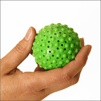
The aim of this activity is to separate a region of interest(ROI) among all the objects in a given image. For an easier implementation of this, it is suggested that the ROI possess a single color. The image I used is shown below with ROI cropped.

The first thing to do here is to crop out the monochromatic region of interest which is the green spiky ball. Then I get the normalized chromaticity coordinates by dividing each R,G and B values in the matrix by their corresponding sum of both the entire image and the ROI. Then before obtaining the probability that the r and g values of every pixel belong to the ROI(p(r) and p(g) respectively, I first obtained the mean and standard deviation of the R and G matrix of the entire image since they values are relevant to the probability distribution.
After applying the probability distribution on each R and G matrix, we get the following images.

(From left to right) P(r) and P(g)
The closer to white pixels suggests that there is a very high probability that those areas would belong to ROI, otherwise they are of less importance with respect to the ROI. If we multiply both of these images we get the figure below. We can still observe here that even though the hand is of less importance with respect to the ROI, the white background still contains green values to it so that it is slightly close in color to the spiky ball. To further remove the white as belonging to the ROI, I binarized the image. It is now shown below.
 Notice here the entire separation of the spiky ball with the white background.
Now, using another technique of ROI separation, we first make a 2D histogram of the original image by just following the code presented in Mam Jing’s lecture. We also compare the derived histogram with the rg chromaticity diagram. This is shown below.
 We take note here that the histogram is rotated 90degress CCW so that their origins will be the same. We can observe that area where non-zero values are found is located in the greenish part of the rg chromaticity diagram like we espected since we get the histogram of a green spiky ball. The histogram by the way is 32x32pixels. Now, like in the backprojection of the previous activity, we are to translate to the image the histogram the histogram shown. This is done by getting the r & g values of the original image. These values just range from 0-1, and since we are to locate it in the histogram, we must first rescale it from 1-32. It is very important to note here that the value of zero for the r and g is prohibited since they will serve as pixel locations in the histogram. What I did was to convert all zeros to one.Now, I took the value of the rescaled r as the x-axis of my histogram and rescaled g as the y-axis. If there are 200×200 values of r’s and g’s, then there will also be 200×200 points from the histogram values which I will place in the same position as my r and g. Upon doing this, i get the image below.
 We can stll see here that ROI encompasses even the background since it is white. The problem here is that although there is some degree of distinction between the white background and the ball but since it peaked out into the white parts thresholding will be difficult.But then I still can clearly separate it from the background by translating the values of the background into near zero or zero itself.
I guess the first part ROI separation is easier to code and gives a reliable result. Still, the second approach is good but i had a hard time doing it so that I obtained this bias. Anyway, I thank mam for helping me in figuring out and debugging the code for my histogram backprojection.
It would be fair enough to give myself a grade of 9 for this activity since all concepts had been clear to me. Only that small programming details have been ignored by oversimplification of concept.
