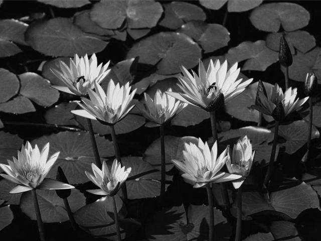
In this activity, I will be compressing the image of water lilies which i got from the sample pictures of my computer. This is essentially an RGB image, and it was converted to grayscale by adding up the matrix of red, green and blue and dividing it by the maximum of these three values which is 3. The original RGB and the grayscale conversion is presented below.
From the grayscale image of size 600×800, it was partitioned into 10×10 matrices which now becomes 60×80, 10×10 matrices. Code is shown.
k=0;
for r = 1:60
for c = 1:80
itemp = I(((10*r-9):(10*r)),((10*c-9):(10*c)));
xtemp = itemp(:);
k = c+(r-1)*80;
x(k,:) = xtemp’;
end;
end;
Then the image x is applied to a pca function in order to get the desired number of lambdas to used for compression. The lambda contribution I chose accumulated to about 95.7% or the first 7 lambdas. Also from this function, we get the ‘basis vectors’ of the image which is also 10×10 in size and from the code, there are a hundred of them. From the information of the number of lambdas to use, I only used the same amount of ‘basis vectors’ to reconstruct the image. PCA code is presented.
[lambda,facpr,comprinc] = pca(x);
y = zeros(100,100);
k=0;
for r=1:10
for c = 1:10
k = c+(r-1)*10;
xtemp = facpr(:,k);
y((10*r-9):(10*r),((10*c-9):(10*c))) = matrix(xtemp,10,10);
end;
end;
//scf(); imshow(y);
Then, from those 7 ‘eigenvectors’, I multipiled the partitioned imaged to each of the eigenvectors and obtained its corresponding sum. This is basically getting the dot product. These numbers or the eigenvalues are stored in a hypermatrix of 7 layers; each layer is obviously 60×80 in size. Code is presented.
hyper_matrix =hypermat([60,80,7]);
for h=1:7
for z=1:60
for a=1:80
new_matrix = I(((10*z-9):(10*z)),((10*a-9):(10*a))).*(y(1:10,((10*h-9):(10*h))));
hyper_matrix(z,a,h) = sum(new_matrix);
end;
end;
end;
From the hypermatrix made, each of the layers having the same location is multipied to the eigenvectors. Then they are summed up and this represents now the 10×10 subimage of the water lilies. The corresponding position in the hypermatrix is the position of the summed vectors in the reconstruction of the image. Dimensionally this is correct since there are 60×80 10×10 ‘s in the original water lily image and so there are also 60×80 in each layer of hypermatrix and the multiplied object(eigen vector) is 10×10 in size. So, bringing the size back to 600×800. Code is shown.
x_comp = [];
for m=1:60
for n=1:80
simple_matrix = zeros(10,10);
for l=1:7
simple_matrix = simple_matrix+hyper_matrix(m,n,l)*(y(1:10,((10*l-9):(10*l))));
x_comp(((10*m -9):(10*m)),((10*n-9):(10*n))) = simple_matrix;
end;
end;
end;
imshow(x_comp);
The resulting compressed image is presented.
We can see that the quality of the picture is reduced and so is the memory size. We can compute the pecent compression by first knowing the number of elements used in the eigenvectors, in this case, it is 7 times a hundred(700) then, also we must know the number of subimages that the images was partitioned, and in this case it amounted to 60×80, 0r 4800 multiplied by the amount of eigenvalues used per subimage which is seven(7). When we add the two up, we get a value of 34300. The original size of the image is basically the number of pixels it has, it amounted to 600×800 or 480000. Therefore the percent compression obtained in this activity is 34300/480000 or we are able to compress the image by up to 7% its original size.
I tried different approaches during my reconstruction part and this approach takes the least amount of code and so in the same way I was able to compress my code. I would probably deserve a grade of 10 for this. However, I must admit that I copied the image presented by Mam Jing in her lecture. This is convenient since the size is divisible to a 10×10 matrix.


